机器人学导论实验:Training an image classifier
一、实验目的
利用Pytorch在CPU/GPU上训练一个图像分类网络
二、实验步骤
- 加载并预处理 CIFAR-10 数据集,包括划分训练集和测试集,并应用图像变换。
- 定义一个卷积神经网络模型结构。
- 定义损失函数和优化器,并利用训练集对模型进行训练。
- 保存训练好的模型。
- 使用测试集评估模型的性能,包括计算总体准确率以及各个类别的准确率。
三、实验过程
1. 使用pip安装Pytorch
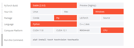
在Pytorch官网找到下载命令,以管理员模式进入命令行,切换到项目根目录输入命令

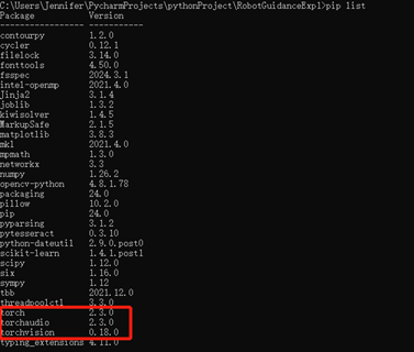
安装成功后,输入pip list确认已安装Pytorch
2. 使用Pytorch官网中训练图像分裂网络的代码,发现报错
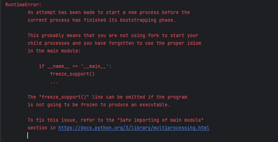
于是在代码前面部分加上

3. 将数据集下载到本地
下载运用网上数据集速度非常慢,因此我们将数据集下载到项目的根目录下
进入官网找到下载方式

将下载的压缩包解压放在新的文件夹data中
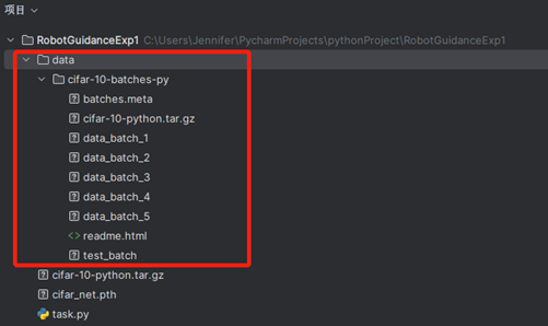
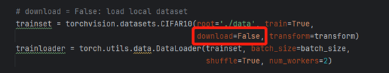
并将download改成false,表示在本地读取数据集
4. 运行代码
加载数据集并进行归一化(normalize)处理,便于后续对模型进行训练1
2
3
4
5
6
7
8
9
10
11
12
13
14
15
16
17
18
19
20
21
22
23
24
25
26
27
28
29
30
31
32
33
34
35
36
37
38
39
40
41
42
43
44
45
46
47
48
49
50
51
52
53
54
55
56
57
58
59
60# 实验:Training an image classifier
# Pytorch训练图像分类网络
# 报告人:韦沁曦
# 学号:2022280210
# 2024.5.15
# First step:
# Load and normalize CIFAR10
# 加载数据集
if __name__ == '__main__':
import torch
import torchvision
import torchvision.transforms as transforms
transform = transforms.Compose(
[transforms.ToTensor(),
transforms.Normalize((0.5, 0.5, 0.5), (0.5, 0.5, 0.5))])
batch_size = 4
# download = False: load local dataset
trainset = torchvision.datasets.CIFAR10(root='./data', train=True,
download=False, transform=transform)
trainloader = torch.utils.data.DataLoader(trainset, batch_size=batch_size,
shuffle=True, num_workers=2)
testset = torchvision.datasets.CIFAR10(root='./data', train=False,
download=True, transform=transform)
testloader = torch.utils.data.DataLoader(testset, batch_size=batch_size,
shuffle=False, num_workers=2)
classes = ('plane', 'car', 'bird', 'cat',
'deer', 'dog', 'frog', 'horse', 'ship', 'truck')
import matplotlib.pyplot as plt
import numpy as np
# functions to show an image
def imshow(img):
img = img / 2 + 0.5 # unnormalize
npimg = img.numpy()
plt.imshow(np.transpose(npimg, (1, 2, 0)))
plt.show()
# get some random training images
dataiter = iter(trainloader)
images, labels = next(dataiter)
# show images
imshow(torchvision.utils.make_grid(images))
# print labels
print(' '.join(f'{classes[labels[j]]:5s}' for j in range(batch_size)))
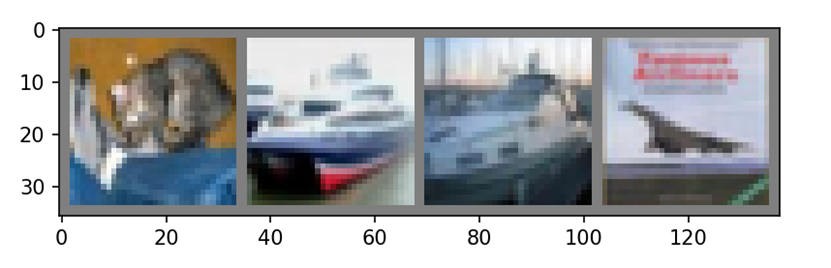
显示处理后图像:
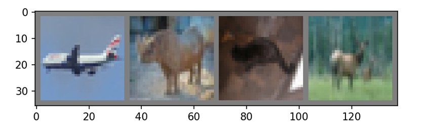
打印真实图像类别

搭建卷积神经网络,定义前向传播为进行两轮卷积、激活、池化,并拉成一个向量
1 | # Second step: |
定义损失函数和优化器SGD
1 | # Third step: |
对网络进行训练
1 | # Fourth step: |
训练结果:
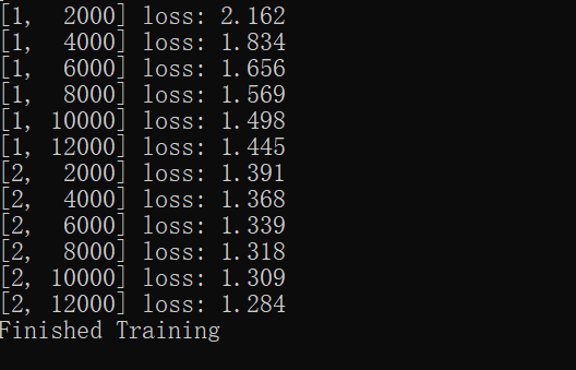
由图可观察到,损失函数逐渐降低
对网络进行测试,计算准确度
1 | # Fifth step: |
显示出预测图像
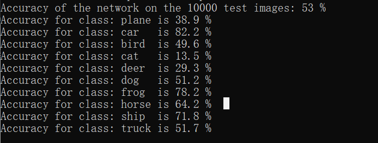
打印真实图像和预测图像的类别,并打印出训练后网络的预测图像准确度
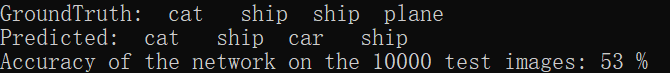
逐行打印每个类别的准确度